6 Data Analysis and Interpretation
6.1 Descriptive statistics: an overview
Introduction
Descriptive statistics are essential tools, particularly when handling large datasets. They simplify and condense our data, making large datasets more ‘digestible’.
With their capability to reflect patterns, trends and relationships, they produce insights that might not be immediately discernible.
Sometimes, descriptive statistics themselves suggest new research questions or fruitful lines of analysis.
Common descriptive statistics
Certain descriptive statistics are the norm in every piece of data analysis that involves quantitative data:
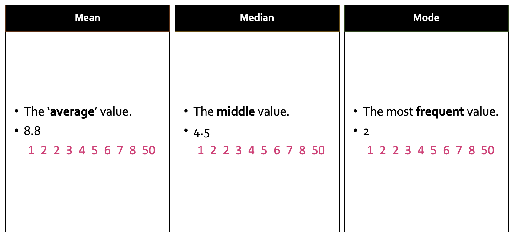
Measures of central tendency, specifically the mean, median, and mode. These measures present the central point or ’typical’ value of a vector.
Beyond central values, understanding the variability within the data is also important. Range and standard deviation are different ways of measuring this variability, and allow us to evaluate the extent of data deviation from the average.
The shape of data distribution (symmetrical, left-skewed, or right-skewed) gives more context about the dataset’s characteristics.
Measures of central tendency
In the following image, three different ways of measuring ‘central tendency’ are shown. Note the difference in each, which in turn tells us something important about the vector.
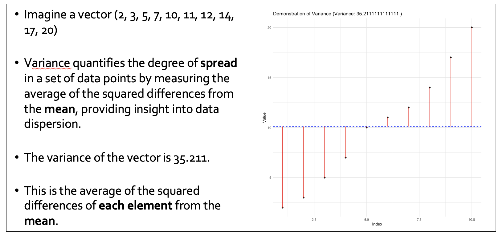
Measures of variability
Variability is the ‘spread’ of the data points in a vector. Higher variability = greater spread around the mean. We are less certain that the mean represents our data.
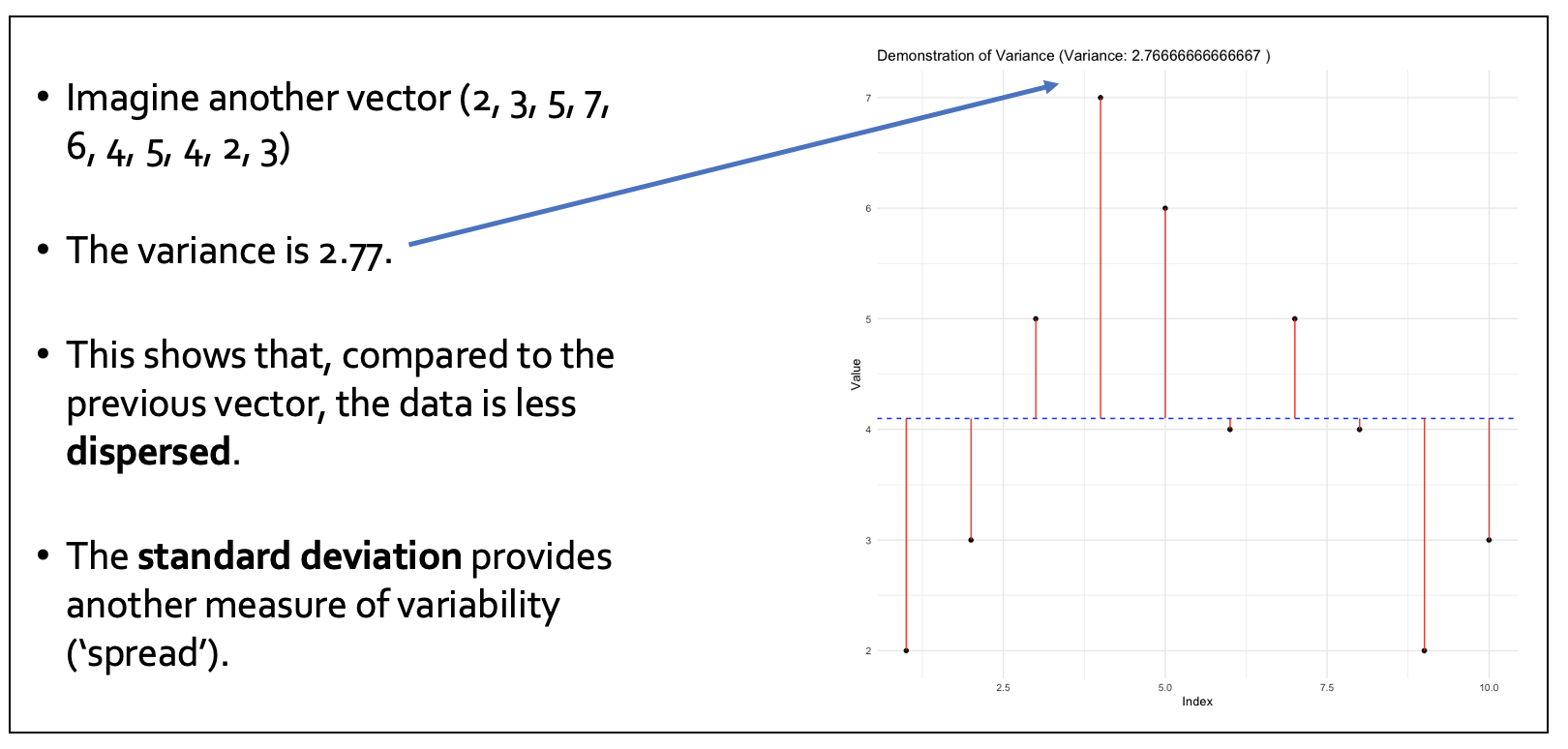
In this example the variability is smaller, so the values are closer to the mean in general.
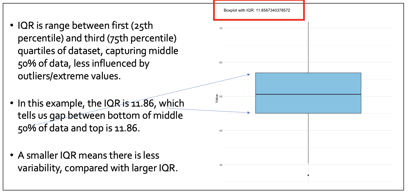
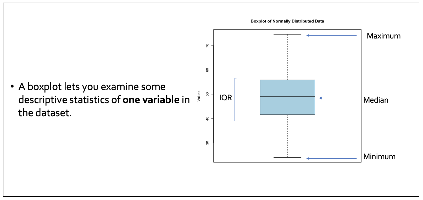
The IQR (inter-quartile range) is another useful descriptive statistic to explore:
Measures of ‘shape’ (distribution)
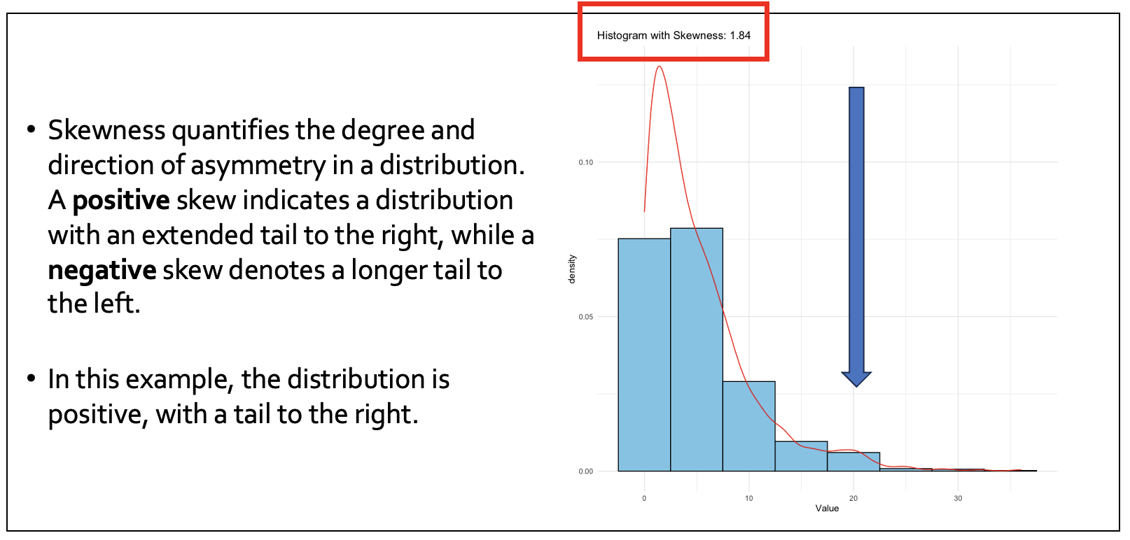
We also need to explore the shape, or ‘distribution’, of our data using ‘skewness’.
Here’s an example of a positive skew - the tail is to the right (i.e. the distribution is ‘skewed’ to the left).
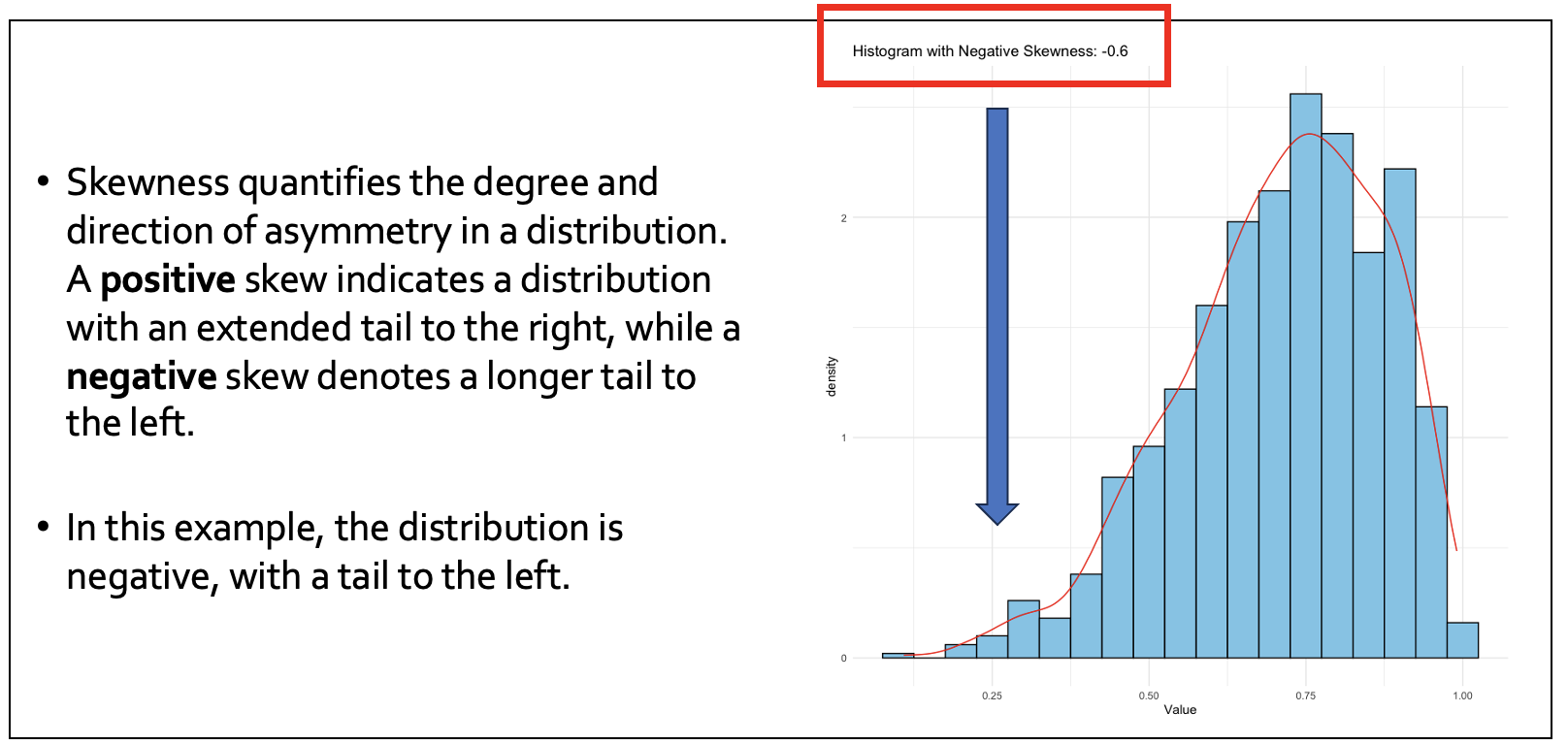
The following is an example of a negative skew - the tail is to the left and the values are skewed to the right.
Visualisation: bringing data to life
Plots and figures based on descriptive statistics really help us understand our data by providing a tangible representation of the data. They’re often much easier to grasp quickly than tables.
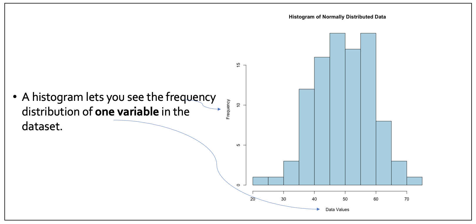
- Bar charts and histograms are useful, especially when illustrating the distribution of data, be it categorical or continuous. They also allow for easy spotting of patterns or outliers.
- Box plots offer a snapshot of data spread and central tendency, while also flagging potential outliers.
- Pie charts, though less common, are useful for displaying the relative proportions of different categories, painting a clear picture of how each segment contributes to the whole.
6.2 Inferential statistics: ‘beyond description’
What are inferential statistics?
Moving on from descriptive statistics, ‘inferential statistics’ act as a bridge that allow us to draw conclusions about a larger population from a smaller sample.
Their predictive power is critical, allowing us to make generalisations and estimations about populations.
They play a key role in estimating population parameters, helping researchers to understand the characteristics of populations rather than just individuals or groups.
They provide a structured framework for hypothesis testing, enabling us to systematically evaluate and make conclusions regarding population attributes based on sample data.
The process of hypothesis testing
Hypothesis testing begins with formulating the null and alternative hypotheses, which respectively represent the status quo and the claim to be tested.
Following this, a test statistic is derived from the sample data, which then serves as a basis for drawing inferences about the broader population.
The final step involves making an informed decision, wherein the null hypothesis is either rejected or retained. This decision hinges on the calculated p-value and a predetermined significance level, often denoted as alpha.
The null hypothesis is a basic concept in statistics that assumes there is no significant difference or effect in a particular situation until proven otherwise. Think of it like this: Imagine you’re saying that a new type of energy drink doesn’t actually change how much energy people feel. That’s your null hypothesis. You’re starting with the assumption that the drink doesn’t do anything special. Then, you conduct experiments or gather data to test if your assumption is wrong. If your data shows that people really do feel more energetic after drinking it, then you can reject the null hypothesis, meaning you’ve found evidence that the drink might actually have an effect. If not, then you haven’t found enough evidence to say the drink does anything, so the null hypothesis remains standing.
Confidence intervals: quantifying uncertainty
Confidence intervals are critical in estimating population parameters. They delineate a range in which the actual population parameter is likely to be located.
The breadth of this interval signifies the precision of the estimate: narrower intervals denote greater precision.
Additionally, the level of confidence, commonly set at 95%, provides a probabilistic interpretation, reflecting the certainty that the interval encompasses the true parameter.
Confidence intervals are like a range that gives us a good guess about where a certain number, like an average, actually falls. Imagine you’re trying to figure out the average height of all the players in a league. It’s tough to measure every single player, so you measure a smaller group and calculate their average height.
Now, you know this average might not be exactly right for all players, so you use confidence intervals to make a safe bet about the range where the true average height probably is. For example, you might end up saying, “I’m 95% confident that the average height of all players is between 5 feet 9 inches and 6 feet 2 inches.”
This doesn’t mean 95% of players are in this height range, but rather you’re 95% sure the true average height of everyone is somewhere in this range. Confidence intervals give us a way to show how certain we are about our estimates, acknowledging that we can’t always measure everything perfectly.
Significance testing: measuring statistical ‘strength’
The p-value is at the heart of significance testing. It’s a metric that quantifies the evidence against the null hypothesis.
A smaller p-value signals a stronger case against the null hypothesis. The alpha level, typically set at 0.05, acts as a cutoff for determining the threshold for statistical significance.
Rejecting the null hypothesis when it is true, or failing to reject it when it is false, can lead to Type I and Type II errors, respectively. Recognising and balancing these errors is crucial in statistical decision-making.
Type 1 and Type 2 errors are like making mistakes in guessing, but in different ways.
Type 1 Error: Imagine you’re playing a game where you guess if a coin flip will land heads or tails. A Type 1 Error is like when you wrongly guess ‘heads’ and it turns out to be ‘tails’. In science, it’s like saying there’s a special effect or difference when there really isn’t one. For example, if you conduct an experiment and wrongly conclude that a new medicine works when it actually doesn’t, that’s a Type 1 Error. You’re seeing something that isn’t there.
Type 2 Error: This is the opposite. Using the coin game example, a Type 2 Error is like not guessing ‘heads’ when it actually lands on heads. In scientific terms, it’s when you miss seeing an effect or difference that is really there. For example, if you test a medicine and conclude that it doesn’t work, but it actually does, you’ve made a Type 2 Error. You’re missing something that is there.
A Type 1 Error is a “false positive” – thinking you’ve found something when you haven’t. A Type 2 Error is a “false negative” – not recognising something that is there.
6.3 Common challenges in data analysis
The term ‘garbage in, garbage out’ is useful to remember when embarking on quantitative analysis. No matter how complex or engaging your statistical analysis, if the data is not of high quality, the results are at best questionable and at worst useless.
It’s important to consider the following before conducting any quantitative analysis (these were introduced in B1700, but are worth revising.)
Missing Data
One of the first challanges often encountered in data analysis is the issue of missing data. Addressing this requires a range of strategies.
Data imputation is a useful technique, where missing values are ‘reasonably’ estimated and replaced based on the patterns observed in available data (for example, with the mean value).
Another approach is outright deletion of observations/rows that contain missing values. However, this tactic can be a double-edged sword, potentially skewing results if the absent data isn’t randomly missing and possibly resulting in significant removal of data that might still be useful.
Thus, it’s important to discern the nature of ‘missingness’. Analysing its pattern to determine whether it’s a random occurrence or stems from a systematic bias can suggest the most appropriate course of action.
Outliers
Outliers, or data points that diverge sharply from the rest, can often adversely impact our analysis.
Detecting these anomalies is the first step, and this can be achieved through visual tools like box plots or more rigorous statistical methods such as Z-scores (covered in B1700).
Once identified, it’s crucial to weigh their potential impact on the overall analysis. Based on their significance and nature, analysts can opt for various strategies, ranging from transforming the data to make outliers less pronounced, to deleting them, or even imputing values in certain cases.
Validity and reliability
For any data analysis to stand the test of scrutiny, it must be both valid and reliable.
Construct validity is critical, ensuring that the tools or measures employed in data collection are genuinely reflective of the intended concepts. Does your measure ‘capture’ what you intend it to?
At the same time, reliability highlights the need for consistency. The same measurements, when taken at different times or scenarios, should yield similar results.
Balancing this with validity, analysts must strike a balance between internal validity, which concentrates on causal relationships, and external validity, which extrapolates these findings to broader contexts.
We will return to these concepts later in this module.
Ethics in analysis
Finally, when thinking about research methods, ethics isn’t merely an afterthought but a crucial consideration. As you know, the importance of data privacy looms increasingly large.
Also, the issue of bias is ever-present. Vigilance is required to sidestep and minimize biases during every phase, from data collection to its eventual interpretation.
Finally, we need to remember the importance of transparency and accountability in all our work, including how we analyse data. When writing code, for example, always assume that someone else will want to see it at a later date.